确定边界
最后就可以通过获取的样本数据,确定边界了。
def determineBounds[K : Ordering : ClassTag]( candidates: ArrayBuffer[(K, Float)], partitions: Int): Array[K] = { val ordering = implicitly[Ordering[K]] // 数据格式为(key,权重) val ordered = candidates.sortBy(_._1) val numCandidates = ordered.size val sumWeights = ordered.map(_._2.toDouble).sum val step = sumWeights / partitions var cumWeight = 0.0 var target = step val bounds = ArrayBuffer.empty[K] var i = 0 var j = 0 var previousBound = Option.empty[K] while ((i < numCandidates) && (j < partitions - 1)) { val (key, weight) = ordered(i) cumWeight += weight if (cumWeight >= target) { // Skip duplicate values. if (previousBound.isEmpty || ordering.gt(key, previousBound.get)) { bounds += key target += step j += 1 previousBound = Some(key) } } i += 1 } bounds.toArray } |
直接看代码,还是有些晦涩难懂,我们举个例子,一步一步解释下:
按照上面的算法流程,大致可以理解:
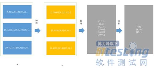
抽样-->确定边界(排序)
首先对spark有一定了解的都应该知道,在spark中每个RDD可以理解为一组分区,这些分区对应了内存块block,他们才是数据最终的载体。那么一个RDD由不同的分区组成,这样在处理一些map,filter等算子的时候,就可以直接以分区为单位并行计算了。直到遇到shuffle的时候才需要和其他的RDD配合。
在上面的图中,如果我们不特殊设置的话,一个RDD由3个分区组成,那么在对它进行groupbykey的时候,就会按照3进行分区。
按照上面的算法流程,如果分区数为3,那么采样的大小为:
val sampleSize = math.min(20.0 * partitions, 1e6)
即采样数为60,每个分区取60个数。但是考虑到数据倾斜的情况,有的分区可能数据很多,因此在实际的采样时,会按照3倍大小采样:
val sampleSizePerPartition = math.ceil(3.0 * sampleSize / rdd.partitions.size).toInt
也就是说,最多会取60个样本数据。
然后就是遍历每个分区,取对应的样本数。
val sketched = rdd.mapPartitionsWithIndex { (idx, iter) =>
val seed = byteswap32(idx ^ (shift << 16))
val (sample, n) = SamplingUtils.reservoirSampleAndCount(
iter, sampleSizePerPartition, seed)
//包装成三元组,(索引号,分区的内容个数,抽样的内容)
Iterator((idx, n, sample))
}.collect()
然后检查,是否有分区的样本数过多,如果多于平均值,则继续采样,这时直接用sample 就可以了
sketched.foreach { case (idx, n, sample) => if (fraction * n > sampleSizePerPartition) { imbalancedPartitions += idx } else { // The weight is 1 over the sampling probability. val weight = (n.toDouble / sample.size).toFloat for (key <- sample) { candidates += ((key, weight)) } } } if (imbalancedPartitions.nonEmpty) { // Re-sample imbalanced partitions with the desired sampling probability. val imbalanced = new PartitionPruningRDD(rdd.map(_._1), imbalancedPartitions.contains) val seed = byteswap32(-rdd.id - 1) //基于RDD获取采样数据 val reSampled = imbalanced.sample(withReplacement = false, fraction, seed).collect() val weight = (1.0 / fraction).toFloat candidates ++= reSampled.map(x => (x, weight)) } |
取出样本后,就到了确定边界的时候了。
注意每个key都会有一个权重,这个权重是 【分区的数据总数/样本数】
RangePartitioner.determineBounds(candidates, partitions)
首先排序val ordered = candidates.sortBy(_._1),然后确定一个权重的步长
val sumWeights = ordered.map(_._2.toDouble).sum
val step = sumWeights / partitions
基于该步长,确定边界,最后就形成了几个范围数据。
然后分区器形成二叉树,遍历该数确定每个key对应的分区id
partition = binarySearch(rangeBounds, k)
实践 —— 自定义分区器
自定义分区器,也是很简单的,只需要实现对应的两个方法就行:
public class MyPartioner extends Partitioner { @Override public int numPartitions() { return 1000; } @Override public int getPartition(Object key) { String k = (String) key; int code = k.hashCode() % 1000; System.out.println(k+":"+code); return code < 0?code+1000:code; } @Override public boolean equals(Object obj) { if(obj instanceof MyPartioner){ if(this.numPartitions()==((MyPartioner) obj).numPartitions()){ return true; } return false; } return super.equals(obj); } } |
使用的时候,可以直接new一个对象即可。
pairRdd.groupbykey(new MyPartitioner())