为了简单起见这里将使用递归来创建树节点,虽然递归不是一个完美的实现,但是对于解释原理他是最直观的。
首先导入库:
import pandas as pd
import numpy as np
import matplotlib.pyplot as plt
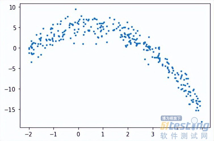
首先需要创建训练数据,我们的数据将具有独立变量(x)和一个相关的变量(y),并使用numpy在相关值中添加高斯噪声,可以用数学表达为:
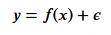
这里的 是噪声。代码如下所示。
def f(x):
mu, sigma = 0, 1.5
return -x**2 + x + 5 + np.random.normal(mu, sigma, 1)
num_points = 300
np.random.seed(1)
x = np.random.uniform(-2, 5, num_points)
y = np.array( [f(i) for i in x] )
plt.scatter(x, y, s = 5)
回归树
在回归树中是通过创建一个多个节点的树来预测数值数据的。 下图展示了一个回归树的树结构示例,其中每个节点都有其用于划分数据的阈值。
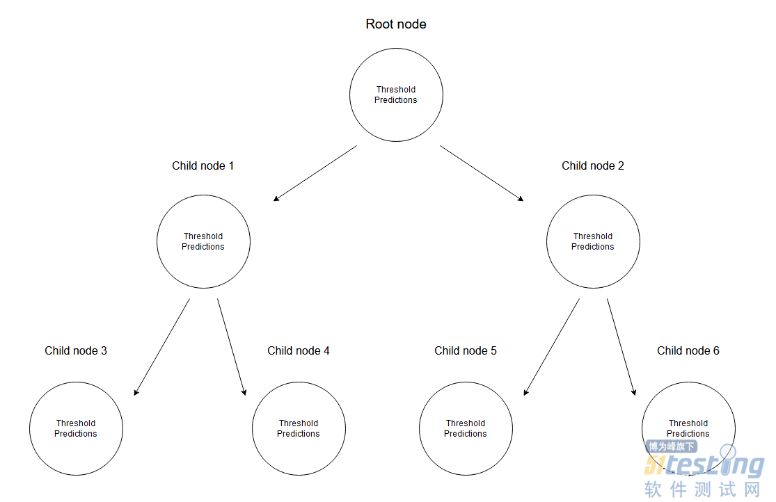
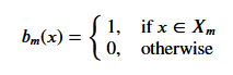
给定一组数据,输入值将通过相应的规格达到叶子节点。 达到节点M的所有输入值可以用X的子集表示。从数学上讲,让我们用一个函数表达此情况,如果给定的输入值达到节点M,则可以给出1个,否则为0。
找到分裂数据的阈值:通过在每个步骤中选择2个连续点并计算其平均值来迭代训练数据。 计算的平均值将数据分为两个的阈值。
首先让我们考虑随机阈值以演示任何给定的情况。
threshold = 1.5
low = np.take(y, np.where(x < threshold))
high = np.take(y, np.where(x > threshold))
plt.scatter(x, y, s = 5, label = 'Data')
plt.plot([threshold]*2, [-16, 10], 'b--', label = 'Threshold line')
plt.plot([-2, threshold], [low.mean()]*2, 'r--', label = 'Left child prediction line')
plt.plot([threshold, 5], [high.mean()]*2, 'r--', label = 'Right child prediction line')
plt.plot([-2, 5], [y.mean()]*2, 'g--', label = 'Node prediction line')
plt.legend()
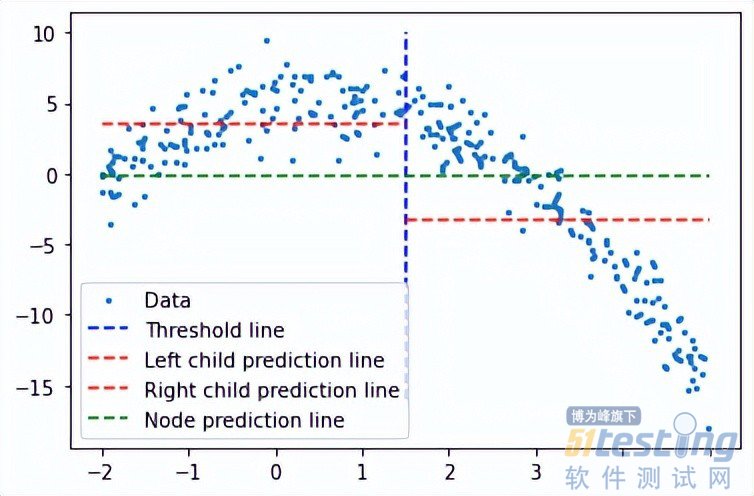
蓝色垂直线表示单个阈值,我们假设它是任意两点的均值,并稍后将其用于划分数据。
我们对这个问题的第一个预测是所有训练数据(y轴)的平均值(绿色水平线)。而两条红线是要创建的子节点的预测。
很明显这些平均值都不能很好地代表我们的数据,但它们的差异也是很明显的:主节点预测(绿线)得到所有训练数据的均值,我们将其分为2个子节点,这2个子节点有自己的预测(红线)。与绿线相比这2个子节点更好地代表了它们对应的训练数据。回归树就是将不断地将数据分成2个部分——从每个节点创建2个子节点,直到达到给定的停止值(这是一个节点所能拥有的最小数据量)。它会提前停止树的构建过程,我们将其称为预修剪树。
为什么会有早停的机制?如果我们要继续进行分配直到节点只有一个值是,这创建一个过度拟合的方案,每个训练数据都只能预测自己。
说明:当模型完成时,它不会使用根节点或任何中间节点来预测任何值;它将使用回归树的叶子(这将是树的最后一个节点)进行预测。
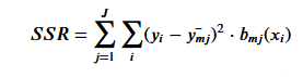
为了得到最能代表给定阈值数据的阈值,我们使用残差平方和。它可以在数学上定义为:
让我们看看这一步是如何工作的。
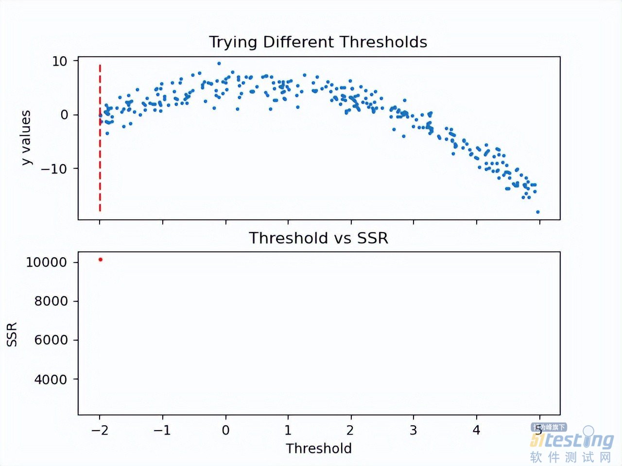
既然计算了阈值的SSR值,那么可以采用具有最小SSR值的阈值。使用该阈值将训练数据分为两个(低和高部分),其中其中低部分将用于创建左子节点,高部分将用于创建右子节点。
def SSR(r, y):
return np.sum( (r - y)**2 )
SSRs, thresholds = [], []
for i in range(len(x) - 1):
threshold = x[i:i+2].mean()
low = np.take(y, np.where(x < threshold))
high = np.take(y, np.where(x > threshold))
guess_low = low.mean()
guess_high = high.mean()
SSRs.append(SSR(low, guess_low) + SSR(high, guess_high))
thresholds.append(threshold)
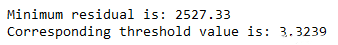
print('Minimum residual is: {:.2f}'.format(min(SSRs)))
print('Corresponding threshold value is: {:.4f}'.format(thresholds[SSRs.index(min(SSRs))]))
在进入下一步之前,我将使用pandas创建一个df,并创建一个用于寻找最佳阈值的方法。所有这些步骤都可以在没有pandas的情况下完成,这里使用他是因为比较方便。
df = pd.DataFrame(zip(x, y.squeeze()), columns = ['x', 'y'])
def find_threshold(df, plot = False):
SSRs, thresholds = [], []
for i in range(len(df) - 1):
threshold = df.x[i:i+2].mean()
low = df[(df.x <= threshold)]
high = df[(df.x > threshold)]
guess_low = low.y.mean()
guess_high = high.y.mean()
SSRs.append(SSR(low.y.to_numpy(), guess_low) + SSR(high.y.to_numpy(), guess_high))
thresholds.append(threshold)
if plot:
plt.scatter(thresholds, SSRs, s = 3)
plt.show()
return thresholds[SSRs.index(min(SSRs))]
创建子节点
在将数据分成两个部分后就可以为低值和高值找到单独的阈值。需要注意的是这里要增加一个停止条件;因为对于每个节点,属于该节点的数据集中的点会变少,所以我们为每个节点定义了最小数据点数量。如果不这样做,每个节点将只使用一个训练值进行预测,会导致过拟合。
可以递归地创建节点,我们定义了一个名为TreeNode的类,它将存储节点应该存储的每一个值。使用这个类我们首先创建根,同时计算它的阈值和预测值。然后递归地创建它的子节点,其中每个子节点类都存储在父类的left或right属性中。
在下面的create_nodes方法中,首先将给定的df分成两部分。然后检查是否有足够的数据单独创建左右节点。如果(对于其中任何一个)有足够的数据点,我们计算阈值并使用它创建一个子节点,用这个新节点作为树再次调用create_nodes方法。
class TreeNode():
def __init__(self, threshold, pred):
self.threshold = threshold
self.pred = pred
self.left = None
self.right = None
def create_nodes(tree, df, stop):
low = df[df.x <= tree.threshold]
high = df[df.x > tree.threshold]
if len(low) > stop:
threshold = find_threshold(low)
tree.left = TreeNode(threshold, low.y.mean())
create_nodes(tree.left, low, stop)
if len(high) > stop:
threshold = find_threshold(high)
tree.right = TreeNode(threshold, high.y.mean())
create_nodes(tree.right, high, stop)
threshold = find_threshold(df)
tree = TreeNode(threshold, df.y.mean())
create_nodes(tree, df, 5)
这个方法在第一棵树上进行了修改,因为它不需要返回任何东西。虽然递归函数通常不是这样写的(不返回),但因为不需要返回值,所以当没有激活if语句时,不做任何操作。
在完成后可以检查此树结构,查看它是否创建了一些可以拟合数据的节点。 这里将手动选择第一个节点及其对根阈值的预测。
plt.scatter(x, y, s = 0.5, label = 'Data')
plt.plot([tree.threshold]*2, [-16, 10], 'r--',
label = 'Root threshold')
plt.plot([tree.right.threshold]*2, [-16, 10], 'g--',
label = 'Right node threshold')
plt.plot([tree.threshold, tree.right.threshold],
[tree.right.left.pred]*2,
'g', label = 'Right node prediction')
plt.plot([tree.left.threshold]*2, [-16, 10], 'm--',
label = 'Left node threshold')
plt.plot([tree.left.threshold, tree.threshold],
[tree.left.right.pred]*2,
'm', label = 'Left node prediction')
plt.plot([tree.left.left.threshold]*2, [-16, 10], 'k--',
label = 'Second Left node threshold')
plt.legend()
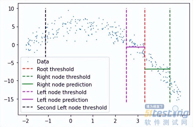
这里看到了两个预测:
· 第一个左节点对高值的预测(高于其阈值)
· 第一个右节点对低值(低于其阈值)的预测
这里我手动剪切了预测线的宽度,因为如果给定的x值达到了这些节点中的任何一个,则将以属于该节点的所有x值的平均值表示,这也意味着没有其他x值参与 在该节点的预测中(希望有意义)。
这种树形结构远不止两个节点那么简单,所以我们可以通过如下调用它的子节点来检查一个特定的叶子节点。
tree.left.right.left.left
这当然意味着这里有一个向下4个子结点长的分支,但它可以在树的另一个分支上深入得多。
预测
我们可以创建一个预测方法来预测任何给定的值。
def predict(x):
curr_node = tree
result = None
while True:
if x <= curr_node.threshold:
if curr_node.left: curr_node = curr_node.left
else:
break
elif x > curr_node.threshold:
if curr_node.right: curr_node = curr_node.right
else:
break
return curr_node.pred
预测方法做的是沿着树向下,通过比较我们的输入和每个叶子的阈值。如果输入值大于阈值,则转到右叶,如果小于阈值,则转到左叶,以此类推,直到到达任何底部叶子节点。然后使用该节点自身的预测值进行预测,并与其阈值进行最后的比较。
使用x = 3进行测试(在创建数据时,可以使用上面所写的函数计算实际值。-3**2+3+5 = -1,这是期望值),我们得到:
predict(3)
# -1.23741
计算误差
这里用相对平方误差验证数据:
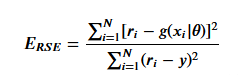
def RSE(y, g):
return sum(np.square(y - g)) / sum(np.square(y - 1 / len(y)*sum(y)))
x_val = np.random.uniform(-2, 5, 50)
y_val = np.array( [f(i) for i in x_val] ).squeeze()
tr_preds = np.array( [predict(i) for i in df.x] )
val_preds = np.array( [predict(i) for i in x_val] )
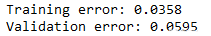
print('Training error: {:.4f}'.format(RSE(df.y, tr_preds)))
print('Validation error: {:.4f}'.format(RSE(y_val, val_preds)))
可以看到误差并不大,结果如下:
概括的步骤:

更深入的模型
一个更适合回归树模型的数据:因为我们的数据是多项式生成的数据,所以使用多项式回归模型可以更好地拟合。我们更换一下训练数据,把新函数设为:
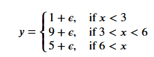
def f(x):
mu, sigma = 0, 0.5
if x < 3: return 1 + np.random.normal(mu, sigma, 1)
elif x >= 3 and x < 6: return 9 + np.random.normal(mu, sigma, 1)
elif x >= 6: return 5 + np.random.normal(mu, sigma, 1)
np.random.seed(1)
x = np.random.uniform(0, 10, num_points)
y = np.array( [f(i) for i in x] )
plt.scatter(x, y, s = 5)
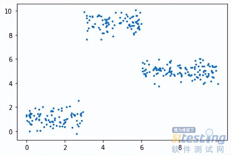
在此数据集上运行了上面的所有相同过程,结果如下:

比我们从多项式数据中获得的误差低。
最后共享一下上面动图的代码:
import pandas as pd
import numpy as np
import matplotlib.pyplot as plt
from matplotlib.animation import FuncAnimation
#===================================================Create Data
def f(x):
mu, sigma = 0, 1.5
return -x**2 + x + 5 + np.random.normal(mu, sigma, 1)
np.random.seed(1)
x = np.random.uniform(-2, 5, 300)
y = np.array( [f(i) for i in x] )
p = x.argsort()
x = x[p]
y = y[p]
#===================================================Calculate Thresholds
def SSR(r, y): #send numpy array
return np.sum( (r - y)**2 )
SSRs, thresholds = [], []
for i in range(len(x) - 1):
threshold = x[i:i+2].mean()
low = np.take(y, np.where(x < threshold))
high = np.take(y, np.where(x > threshold))
guess_low = low.mean()
guess_high = high.mean()
SSRs.append(SSR(low, guess_low) + SSR(high, guess_high))
thresholds.append(threshold)
#===================================================Animated Plot
fig, (ax1, ax2) = plt.subplots(2,1, sharex = True)
x_data, y_data = [], []
x_data2, y_data2 = [], []
ln, = ax1.plot([], [], 'r--')
ln2, = ax2.plot(thresholds, SSRs, 'ro', markersize = 2)
line = [ln, ln2]
def init():
ax1.scatter(x, y, s = 3)
ax1.title.set_text('Trying Different Thresholds')
ax2.title.set_text('Threshold vs SSR')
ax1.set_ylabel('y values')
ax2.set_xlabel('Threshold')
ax2.set_ylabel('SSR')
return line
def update(frame):
x_data = [x[frame:frame+2].mean()] * 2
y_data = [min(y), max(y)]
line[0].set_data(x_data, y_data)
x_data2.append(thresholds[frame])
y_data2.append(SSRs[frame])
line[1].set_data(x_data2, y_data2)
return line
ani = FuncAnimation(fig, update, frames = 298,
init_func = init, blit = True)
plt.show()
本文内容不用于商业目的,如涉及知识产权问题,请权利人联系51Testing小编(021-64471599-8017),我们将立即处理